Study population
UKB is a repository of research data sourced from ~ 500,000 UK-wide participants aged around 40–70 years old, recruited from 22 assessment centers during 2006–2010 [28]. We used data collected for each participant from enrollment to March 26, 2021. In brief, data in the UKB repository was grouped into 277 categories, and we retrieved those related to (i) socioeconomic factors (categories 100,066, 100,063, and 100,064); (ii) lifestyle factors (categories 100,058, 100,054, 100,052, 100,051, 100,057, and 143); (iii) environmental pollution factors (categories 114 and 115); (iv) health outcome factors (categories 2002, 100,074, 100,060, 137, and 100,092) (Additional file 1: Table S1) [29]. Note that although an individual’s SES and lifestyle may change over time, we used the baseline survey data to define the socioeconomic and lifestyle status of each participant. A research protocol for our study has obtained all necessary approvals from the UKB’s review committees. We accessed to the UKB cohort consisting of 502,462 individuals. Following Yang and Zhou [30, 31], we removed individuals: (i) who have sex mismatched; (ii) who are redacted and thus do not have a corresponding ID; (iii) who have missing information on socioeconomic factors or other covariates. Finally, we retained 412,258 participants in UKB for subsequent analysis (Fig. 1a).
Fig. 1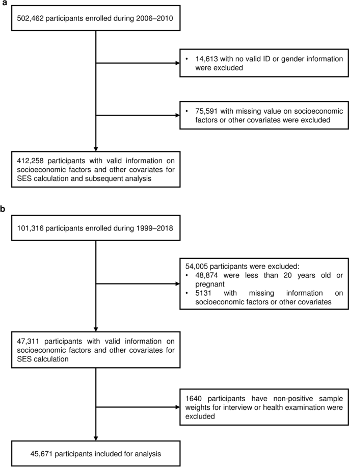
Flowchart of the participants selection in the UK Biobank (a) and US NHANES (b). SES socioeconomic status
In US NHANES, we included 101,316 participants surveyed from 1999 to 2018, and followed Zhang et al. to remove individuals: (i) who were less than 20 years old; (ii) who were pregnant; (iii) who had missing information on socioeconomic factors or other covariates; (iv) who had non-positive sample weights for an interview or health examination in the datasets [32]. Finally, we retained 45,671 participants in US NHANES for subsequent analysis (Fig. 1b). Details about the introduction, the definitions of socioeconomic, lifestyle, and chronic comorbidity factors, and infectious diseases in US NHANES are provided in Additional file 1: Tables S2 and S3, and Additional file 2: Methods.
Assessment of socioeconomic status
We followed Zhang et al. to assess the individual SES based on four variables collected at baseline, including family income level, education qualification, employment status, and health insurance coverage [32]. In particular, however, considering the implementation of the National Health Service, a publicly funded healthcare system in the UK, we used three variables, including the total household income level, education qualification and employment status, rather than the health insurance coverage, to assess the SES of each participant at individual level [33]. For total household income level before tax, participants chose an option from (i) < £18,000; (ii) £18,000–£30,999; (iii) £31,000–£51,999; (iv) £52,000–£100,000; (v) > £100,000; (vi) do not know; and (vii) prefer not to answer. We removed the participants choosing the last two options. Education qualification was recorded as (i) College or University degree; (ii) A levels, AS levels, or equivalent; (iii) O levels, GCSEs, or equivalent; (iv) CSEs or equivalent; (v) NVQ, HND, HNC, or equivalent; (vi) other professional qualifications; and (vii) none of the above (following Zhang et al. [32] we treated it as equivalent to or less than high school diploma); and (viii) prefer not to answer. We removed the individuals choosing the last option. Considering no clear rank order of employment status among candidate options, including (i) in paid employment or self-employed; (ii) retired; (iii) looking after home and/or family; (iv) unable to work because of sickness or disability; (v) unemployed; (vi) doing unpaid or voluntary work; (vii) full or part-time student; (viii) none of the above; and (ix) prefer not to answer, we removed participants choosing the last option and simply regrouped the remaining participants into two groups: employed (those chose (i), (ii), (vi) and (vii)) and unemployed (those chose others). Variable definitions were listed in Additional file 1: Table S1.
Following Zhang et al. [32] we then used latent class analysis (LCA), using multiple observed categorical variables to construct an unmeasured variable (i.e., latent variable), to estimate SES based on the above three variables in UKB. We used R package poLCA (v1.6.0) to implement the LCA procedure, and set the maximum times of iterations to 10,000, and the tolerance value for judging convergence to 1 × 10⁻⁶ [34]. To select a reasonable latent class number, we fitted the different LCA model with 2–10 latent classes. Models failed to converge when the class number is greater than five. We further used Akaike information criterion (AIC), Bayesian information criterion (BIC), and likelihood ratio statistic (G2) for parameter selection, and treated latent class with mean posterior probability higher than 0.7 as classification with acceptable uncertainty (Additional file 1: Table S3 and Additional file 2: Fig. S1). Finally, three latent classes were identified, which respectively represented a high, medium, and low SES according to the item-response probabilities (Additional file 1: Table S3).
In addition, for UKB, we also included the Townsend deprivation index (TDI) as an area level SES, which represents a comprehensive score of four key variables: unemployment, overcrowded household, non-car ownership, and non-home ownership, with a higher score representing higher levels of deprivation [35, 36].
Assessment of lifestyle factors
Following Said et al., Fan et al., and Zhu et al. [37,38,39] we included information on five healthy lifestyle factors collected at baseline, including “no current smoking”, “regular physical activity”, “healthy diet pattern”, “no alcohol consumption”, and “healthy sleep pattern”. In addition, given that drug abuse behavior has been proved a high-risk factor for some infectious diseases [40, 41], we also regarded “no drug use” as the sixth healthy lifestyle factor. We then used the six healthy lifestyle factors to generate a comprehensive lifestyle score.
Lifestyle information in UKB was also obtained through structured questionnaires (Additional file 1: Table S1). “No current smoking” was defined as never smoking or former smoking but had quit for more than 30 years. “No alcohol consumption” was defined as never drinking alcohol. UKB records the use of cannabis, and “No drug use” was defined as never use cannabis. “Regular physical activity” was defined to meet one of the following: (i) from the perspective of frequency, to engage in vigorous physical activity for at least one day and moderate activity for at least five days per week; (ii) from the perspective of time, to exercise of vigorous activity for at least 75 min or moderate activity for 150 min per week. “Healthy diet pattern” includes (i) adequate consumption of fruit, (ii) vegetables, (iii) fish, and (iv) whole grains, but (v) reduced consumption of processed and (vi) unprocessed meats. The specific definition for each pattern was in Additional file 1: Table S1, and we defined a healthy diet pattern as following at least four factors. As for sleep patterns, five sleep factors, including chronotype, duration, insomnia, snoring, and involuntary daytime sleepiness, over the last four weeks were considered and surveyed [38]. “Healthy sleep pattern” was defined as: (i) self-reported as early chronotype; (ii) sleep 7–8 h per day; (iii) rarely suffer from insomnia; (iv) no snoring symptoms; and (v) infrequently doze off or fall asleep involuntarily during the daytime. The specific definition for each pattern was also in Additional file 1: Table S1, and we defined a healthy sleep pattern as following at least four of these five factors.
For each lifestyle factor, we assigned 1 point for a healthy level while 0 points for an unhealthy level. The lifestyle variable was defined as the summation of the six variables and was divided participants into 3 groups: poor group (0–1 point), medium (2–3 points) and healthy (4–6 points).
Assessment of environmental pollution
Environmental pollution information was recorded only in UKB. Following Huang et al. and Furlong et al. [42, 43] we considered eight environmental pollution factors, including particulate matter ≤ 2.5 μm (PM2.5), particulate matter 2.5–10 μm (PM2.5–10), particulate matter ≤ 10 μm (PM10), nitrogen oxides (NOx), and nitrogen dioxide (NO2), noise, distance to nearest major road, and traffic intensity (Additional file 1: Table S1). All environmental pollution factors were estimated by the Small Area Health Statistics Unit as part of the BioSHaRE-EU Environmental Determinants of Health Project. Values of PM2.5, PM2.5–10, PM10, NOx, NO2 and noise were calculated in 2010 using a Land Use Regression (LUR) model developed as part of the European Study of Cohorts for Air Pollution Effects (ESCAPE) and represented annual averages of air pollution in 2010 for the reported residence at enrollment [44, 45]. Specifically, given that impacts of noise usually vary over a time period, a day-evening-night equivalent level with a 5 dB and 10 dB penalty added to the average sound level of noise pollution of the evening (19:00 to 23:00) and night-time (overnight 23:00 to 07:00), respectively. We used weighted average noise exposure level measured over a 24-h period to further analysis [43, 46, 47]. In addition, distance to the nearest major road and traffic intensity were measured based on the local road network from the Ordnance Survey Meridian 2 road network in 2009. We treated the estimated values for 2009 and 2010 as a proxy for a measure of chronic, long-term exposure to environmental pollutants, following previous studies [24, 43]. Note that to facilitate interpretation, we calculated the odds ratio (OR) per 10-unit increase in each environmental pollution factor to reflect its association with infection [43]. To demonstrate the reasonability of this proxy, we also conducted a side analysis using participants enrolled in 2010, which is also a part of sensitivity analyses.
We then created weighted environment pollution score (EPS) through adding measurements of eight environmental pollutants, weighted by the adjusted estimates from multivariable analysis on the prevalence of infectious diseases [48]. The equation is as follows:
$$\begin{array}{c}{EPS}_{i} = \frac{p}{\sum {{\varvec{\beta}}}_{j}}{\sum }_{j = 1}^{p}{{\varvec{\beta}}}_{j}{{\varvec{X}}}_{ij}\#\left(1\right)\end{array}$$
where \(p\) represented the number of environmental pollutants; \({{\varvec{\beta}}}_{j}\) was adjusted coefficients of environmental pollutants \(j\); \({{\varvec{X}}}_{ij}\) and \({EPS}_{i}\) was the measurements of \(j\) th pollution of \(i\) th individual. We also calculated a weighted air pollution score (APS) using PM2.5, PM2.5–10, PM10, NOx, NO2, as done in previous studies to serve as a sensitivity analysis. Note that for the analysis on the association of EPS and APS with infection, we divided the participants into five groups (Q1–Q5) according to the quantiles of the scores, and evaluated the association between score groups and infection, as well as ORs of groups with higher scores (Q2–Q5) to the group with lowest scores.
Assessment of chronic comorbidities
We considered four types of chronic comorbidities, including cardiovascular disease (CVD), diabetes, psychiatric disorders and cancer (Additional file 1: Table S1). We followed Zhu et al. and Said et al. [39, 49] and used diagnosis records in UKB coded by International Classification of Diseases version-10 (ICD-10) to define participants with CVD, diabetes and cancer at baseline. Specifically, we totally defined 35,469 (8.8%) participants with CVD history, including 5055 (1.3%) CAD cases (ICD-9 codes 410–412; ICD-10 codes I21–I23, I24.1, and I25.2), 4824 (1.2%) atrial fibrillation (AF) cases (ICD-9 codes 4273; ICD-10 codes I48), 1945 (0.5%) stroke cases (ICD-9 codes 430, 431, 434, and 436; ICD-10 codes I60, I61, I63, and I64), and 29,294 (7.3%) hypertension cases (ICD-9 codes 401–405; ICD-10 codes I10–I13, I15, O10). We also defined 7922 (2.0%) and 30,176 (7.5%) participants with a history of diabetes (ICD-9 codes 250; ICD-10 codes E10–E14) and cancer (ICD-10 codes C00–D48), respectively. In terms of psychiatric disorders, we followed Davis et al. [50] and considered participants who had self-reported anxiety, depression or bipolar disorder. Specifically, we totally defined 58,381 (14.6%) participants with a history of psychiatric disorders, including 23,079 (5.8%), 45,023 (11.2%) and 1582 (0.4%) with anxiety (field 20,002 codes 1287; field 20,544 codes 15), depression (field 20,002 coded 1286; field 20,126 coded 3–5; field 20,544 codes 11) and bipolar disorder (field 20,002 coded 1291; field 20,126 coded 1–2; field 20,544 codes 10), respectively.
Definition of outcome
In UKB, infectious diseases were also defined according to diagnosis records in UKB coded by the ICD-10 and ICD-9. We used data collected up to March 26, 2021. Referring to the coding terms, we defined a total of 60,771 (14.7%) cases with infectious diseases (ICD-10 codes A00–B99 and J00–J22; ICD-9 codes 001–139 and 480–487). Furthermore, we also defined three subtypes of infectious diseases from it: (i) respiratory infectious diseases (ICD-10 codes A15, A37, A39, B01, B02, B05, B06, B26, and J09–J11; ICD-9 codes 001, 012, 033, 036, 053, 055, 056, 072 and 487) with 2119 (3.5%) cases; (ii) digestive infectious diseases (ICD-10 codes A00–A09, B15, B17.2, B67, B68, B77, B80, and B82; ICD-9 codes 001–009, 0701, and 122) with 15,019 (24.7%) cases; (iii) blood or sexually transmitted infectious diseases (ICD-10 codes A50–A64, B16, B17.1, B18.0, B18.1, B18.2 and B20–B24; ICD-9 codes 0703 and 090–099) with 869 (1.4%) cases, to explore the association of research factors with common infectious diseases types (Additional file 1: Table S1). In addition, we also defined 71,335 participants enrolled in 2010, among whom 9682 (13.6%) were infected, to serve as sensitivity analysis.
Statistical analysis
Baseline characteristics of three SES groups were compared using the unpaired, 2-tailed t test or Mann–Whitney test for continuous variables depending on the data distribution, and the χ2 test was used for categorical variables. Continuous variables are presented as mean (SD) or median (quartile); categorical variables are presented as number (percentage). Second, multivariable logistic regression was used to test association of SES, lifestyle factors, environmental pollution, and chronic comorbidity factors with infectious diseases. We treated age, sex, ethnicity and assessment center as covariates, and reported adjusted OR with 95% confidence intervals (CIs). Third, multiplicative interaction analysis, along with stratified analysis, was used to ask about the moderation effects of SES on association of lifestyle, environmental pollution, and chronic comorbidity factors with infectious diseases. A two-sided P < 0.05 was considered statistically significant. All analyses were performed using the statistical software R 4.1.0 (Lucent Technologies, Jasmine Mountain, USA).
A mediation analysis was conducted to evaluate the proportion mediated by lifestyle, environmental pollution, and chronic comorbidity factors for the association between SES and infectious diseases. Associations of lifestyle, environmental pollution, and chronic comorbidity factors on infections were tested using logistic regression. Associations of SES on individual lifestyle factors were also analyzed using logistic regression, while those of SES on lifestyle scores, EPS and individual environmental pollutant were analyzed using linear regression. All regression analyses were adjusted for age, sex, ethnic and assessment center.
Sensitivity analyses
To ensure the robustness of our result, we considered seven kinds of sensitivity analyses. First, in terms of socioeconomic factors, we additionally considered the TDI as an area level SES variable. We not only directly explored its association with infectious diseases, but also took it as a covariate in the association analysis of individual-level SES on infection. Second, in terms of lifestyle, environmental pollution and chronic comorbidities, we repeated all main analyses conducted in those composite variables for each individual factor. Third, in terms of environmental pollution, we further calculated a weighted APS using five air pollution factors, including PM2.5, PM2.5–10, PM10, NOx, NO2, as done in previous studies [24, 48]. Fourth, in terms of infectious diseases, considering that we took environmental pollutants measurement in 2009 and 2010 as a proxy for chronic, long-term exposure estimation, we also repeated the main analysis in a subset of participants enrolled in 2010. Fifth, given the case–control imbalance in analysis of different infectious diseases subgroups, we performed a propensity score matching (PSM). We treated age, sex, ethnicity and assessment center as matching covariates, and used the nearest neighbor method to make a 1:4 matching. Finally, we additionally used data from US NHANES to validate our main results. We repeated the main analysis in US NHANES, except for those on environmental pollution variables. In particular, due to the application of oversampling in US NHANES survey, we considered sample weights recorded in US NHANES, which indicate a measure of the number of people in the population represented by a specific person, in descriptive and other analysis to obtain accurate point estimates and standard errors. Note that frequency was reported directly based on the sample data (i.e., the 47,311 sampled participants), while other statistics were estimated and reported in a weighted manner. Survey (v 4.1.1) and svrepmisc (v 0.2.2) packages were used to account for the sample weights. Covariates used for US NHANES included age, sex, ethnicity and survey cycle.
Source: news.google.com